
After reading the chapters and completing exercises in Unit 4, the reader will be able to:
Road safety management refers to the process of identifying safety problems, devising potential strategies to combat those safety problems, and selecting and implementing the strategies. Effective safety management is also proactive and looks for ways to prevent safety problems before they arise. High quality safety data should be used to determine the nature of the road safety problems and how best to solve them. As discussed in Unit 3, the clearest and most readily available indicators of road safety problems are crash data. These data can be used to identify safety problems on a large or a small scale. Other data, such as roadway characteristics, traffic volume, citations, and driver history, can be integrated with crash data to assist in identifying safety trends and high priority locations.
Every transportation agency will acknowledge that it does not have perfect data. All data have issues related to accuracy, coverage, timeliness, and other factors. One agency's crash data may have an incomplete record of low severity crashes. Another agency may have very little data on the traffic volume on low volume rural roads. However, data quality issues should not prevent a transportation agency from using the data to drive its safety management efforts. Even while the agency strives to improve its data, the data on hand should be used in the process of identifying safety problems and devising solutions to those problems.
A numerical metric used to monitor changes in system condition and performance against established visions, goals, and objectives.
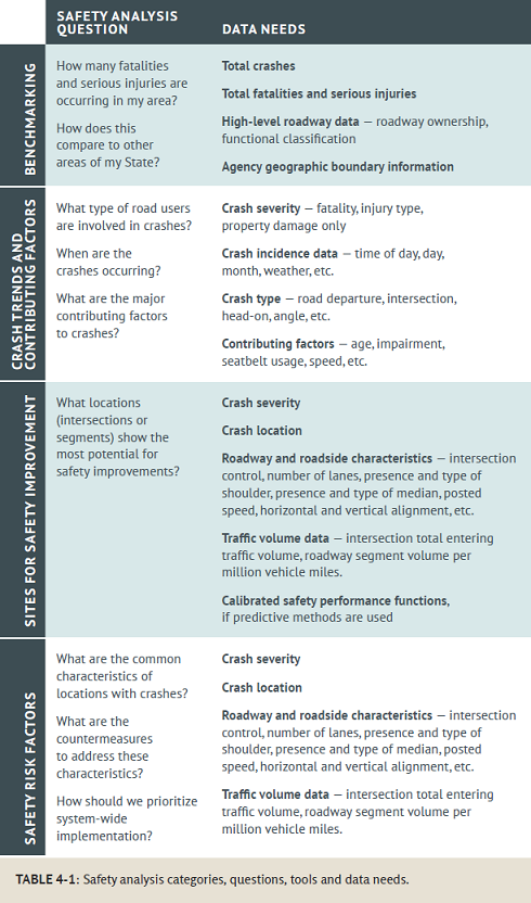
High quality safety analysis demands high quality data. Unfortunately, poor data availability and low quality limit the types of analyses that can be conducted. The data requirements depend on the type of analysis and what safety questions are being asked. Table 4-1 provides examples of various categories of safety analysis and lists the data that would be needed to conduct them.1
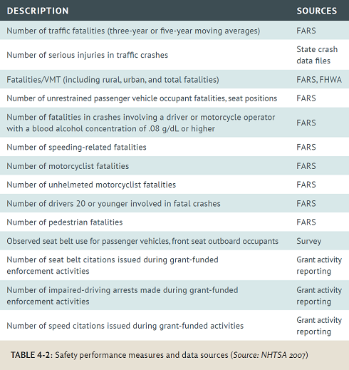
A transportation agency has many types of data at its disposal for identifying safety problems, but the agency must select which type(s) of data will be the performance measures used to identify the road safety emphasis areas. Federal legislation has focused increasingly on fatal crashes and serious injury crashes as performance measures for road safety.
Table 4-2 provides examples of performance measures developed by the National Highway Traffic Safety Administration (NHTSA) and the Governors Highway Safety Association (GHSA) that could be used to identify safety priorities.2 The sources of the data could be State crash data files, the Fatality Analysis Reporting System (FARS), surveys conducted by the State, or grant applications from law enforcement and other departments. The section on Network Screening in Chapter 11 presents a more detailed discussion of crash-based performance measures and how they can be used to identify sites that are high priority for safety treatment.

The safety management process can be viewed in three general components. These components are carried out by the agency (or agencies) responsible for managing the safety of the road system:
Although all road safety management follows the same three general components listed above, the specific steps of the safety management process will be different depending on the scope. The process might be intended to address specific site-level issues, such as crash patterns at high priority intersections, curves, or corridors. On a larger scale, the process might be intended to address system-level issues, such as problems that can be addressed by policies, design standards, or broad ranging campaigns of education or enforcement. The following chapters will discuss safety management for these two levels: Chapter 11 presents site-level safety management; Chapter 12 presents system-level safety management.
Site-level safety management is the process of identifying and addressing safety issues at high priority sites. This contrasts with safety issues that are addressed for an entire transportation system (i.e., all roads in a city, county, or State). System-level safety management is covered in Chapter 12.
A narrowly defined location of interest for safety analysis, such as an intersection, road section, interchange, or midblock crossing.
Agencies responsible for road safety often conduct some form of site-level safety management. They identify particular sites of concern and determine how best to address the safety problems at these priority sites. The methods of identifying priority sites and the safety strategies used to treat the sites differ according to the type of agency. A department of transportation (DOT) may install a sign or pavement marking; a law enforcement agency might increase enforcement in the area of the site. Regardless of the type of agency, it is important to conduct site-level safety management in a manner that uses good analysis methods driven by safety data.
Chapter 10 presented road safety management in terms of three general components:
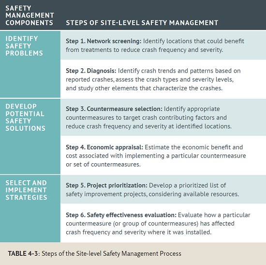
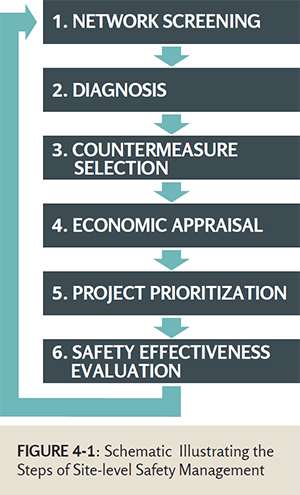
When discussing site-level safety management, these three components can be further divided into six distinct steps. This six-step process is common to the engineering discipline and is presented in Part B of the first edition of the Highway Safety Manual3 (HSM). The process, shown in Figure 4-1, will be the framework for the discussion of site-level safety management in this chapter. The material presented in this chapter is based on the guidance presented in the HSM and material from a series of documents entitled “Reliability of Safety Management Methods” published by FHWA. These FHWA documents provide in-depth guidance and examples on the following topics:
The six steps of the site-level safety management process relate to the three general components of safety management as shown in Table 4-3. Each step is presented in more detail through the following sections in this chapter.
The number of observed crashes per year.
The level of injury severity of the crash as an event, typically determined by the highest severity injury of any person involved in the crash.
The number of observed crashes per unit of traffic volume passing through the location.
Network screening refers to the process of selecting high priority sites that need safety treatment, often through an analysis of crash data. There are many ways in which an agency can use crash data to prioritize sites, ranging from simplistic methods, which are easy to understand and implement but can be inaccurate or ineffective, to more advanced methods, which require statistical expertise and more data but provide a better prioritization of sites.
For many years, the most prevalent methods for ranking specific sites for safety improvements were based on historical crash data alone. Many agencies still use these methods to allocate their road safety funds. Agencies that prioritize sites by historical crash frequency identify those sites that have the highest number of crashes in a certain time period (typically three to five years). This serves to assist agencies in addressing the magnitude of the problem, that is, attempting to address the highest number of crashes. By its nature, this method typically identifies sites that have high amounts of traffic (either vehicles, pedestrians, or other road users). However, this method may miss abnormally hazardous sites that do not present a relatively large number of crashes. Another variation of the crash frequency method uses crash severity, in which agencies weight the crash frequency by giving greater weight to higher severity crashes. This method counteracts some of the bias in the crash frequency method. For example, a general high crash frequency may prioritize a busy intersection that has many crashes, but a closer examination reveals that most crashes are low speed, low severity rear-end crashes. The crash severity method would lower the priority of this intersection in favor of other sites where more serious crashes occur.
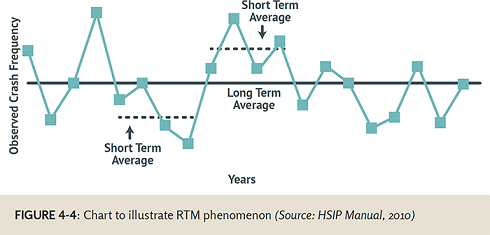
The fact that a short term examination of crash history at a location is likely inaccurate (e.g., lower or higher than its true safety performance). When a longer time period of crash history is examined, the crash frequency will “regress” to its “mean” and provide a better picture of the long term average crash frequency.
Some agencies prioritize sites by the historical crash rate. This method incorporates traffic volume to augment the crash data. The crash frequency at a site is divided by the traffic volume—either the annual average daily traffic (for road segments), total entering volume (for vehicle traffic at intersections), or other volumes, such as pedestrian crossing volume. The typical unit for this method is crashes per 100 million vehicle miles traveled for road segments or crashes per 100 million entering vehicles for intersections. Crash rate in these units is calculated as:
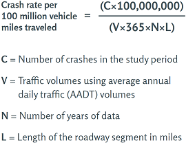
This approach of prioritizing sites by crash rate serves to counteract the bias of crash frequency that overly prioritizes sites with high volume, since higher volume decreases the crash rate. However, it may inefficiently prioritize sites with very low volumes.
Road Segment A:
A three-mile section of road that has had four crashes over five years and has a traffic volume of 4,000 vehicles per day.
Road Segment B:
A three-mile section of road that has had 10 crashes over five years and has a traffic volume of 12,000 vehicles per day.
If an agency is comparing these segments based on crash frequency, they would prioritize road segment B for having 10 crashes compared to road segment A which had four crashes.
If comparing these segments based on crash rate, the agency would calculate the crash rate of road segment A as (4 crashes x 100,000,000) / (4,000 vehicles per day x 365 x 5 years x 3 miles) = 18.2 crashes per 100 million vehicle miles traveled. Following the same calculation, road segment B has a rate of 15.2 crashes per 100 million vehicle miles traveled. According to crash rate, the agency would prioritize road segment A. The prioritization of these two segments changes when traffic volume is taken into account.
Agencies might use a combination of these two methods. They may set a minimum crash rate to generate an initial list of priority sites and then prioritize that group by crash frequency or severity. Regardless, these simplistic methods are known to have potential biases. One of the most prevalent biases is that the crash history used to prioritize sites with these methods usually reflects only the short-term trend of crashes. Given that the year-to-year occurrence of crashes at a location is random, it can be the case that a short-term crash history (one to three years) may be relatively high, but in the long run (ten years), the crashes would return to a lower amount, even if no safety improvements were done. This effect creates selection bias or regression-to-the-mean (RTM) bias in the safety analysis of this location.
As the years progressed, many transportation safety professionals recognized that while these simplistic methods did identify sites that benefited from safety improvement, they were not the locations where safety funds could be spent the most effectively. The selection of high crash sites was subject to RTM bias. Also, sites with high numbers of crashes were typically complex and required expensive reconstruction in order to reduce crashes appreciably. The question became, “How could road safety funds be spent in a way that provided the biggest bang for the buck?”
As the science of road safety advanced, researchers developed more advanced approaches for prioritizing sites for safety improvements. Dr. Ezra Hauer pushed forward a movement to identify “sites with promise.”9 The main idea was to identify sites that experienced more crashes than would be expected from a site with that particular set of characteristics. In many cases, these abnormally performing sites could be addressed with low cost safety treatments, such as larger signs or pavement markings with greater visibility. This approach uses statistical regression models that predict crashes for a given set of characteristics. These models demonstrate the advantage of bringing together different types of safety data, which in this case could include crash data, roadway characteristics, and traffic volume.
The frequency of crashes per year that would be predicted for a site based on the result of a crash prediction model, called a safety performance function (SPF).
The most basic of these regression methods calculates predicted crashes. This method requires information about certain geometric and operational characteristics, such as traffic volume, number of lanes, and type of road.
An SPF is developed or calibrated using data from an entire jurisdiction or State, so it is independent of the crash history of the specific site. This means that the predicted crash value is unaffected by the bias caused by RTM. Using SPFs, transportation agencies can predict crash values for many sites and prioritize the sites according to the highest predicted values. Another use of the predictive method is in systemic safety treatments, presented in Chapter 12 under Risk Based Prioritization.
The first edition of the HSM lists several benefits of the predictive method, including:
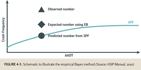
Agencies can also use the predicted crashes in combination with actual crash history at the site of interest to calculate expected crashes. A method called empirical Bayes (EB) brings these two values together to reflect a crash frequency that incorporates the general crash prediction from the SPF with the real world experience of crash history at the site to provide an accurate estimation of how many crashes should be expected at the site (see more detailed discussion of the EB method later in this step). Some agencies may also calculate excess crashes as a measure for site prioritization. This is the difference between the expected crashes and the observed crash frequency at the site.
The key to effective network screening is selecting an appropriate performance measure. Network screening methods should appropriately account for three major factors that can affect the screening outcome:
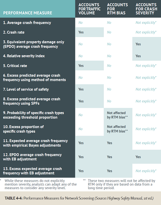
Table 4-4 lists the thirteen performance measures discussed in the HSM with an indication of their ability to account for these major factors. While some measures directly account for crash severity (e.g., relative severity index), analysts can adapt any of the measures to account for crash severity.
As discussed earlier, analysts have traditionally used crash rates to account for differences in traffic volume among sites. Crash rate is the ratio of crash frequency to exposure, which is typically the traffic volume. Crash rates implicitly assume a linear relationship between crash frequency and traffic volume; however, many studies have shown that the relationship between crashes and traffic volume is nonlinear, and the shape of this relationship depends on the type of facility. Nonlinear relationships, such as SPFs, are more appropriate than linear relationships, such as crash rates to account for differences in traffic volume among sites.
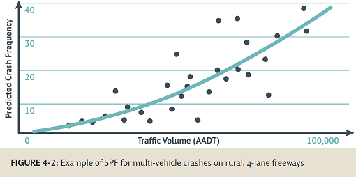
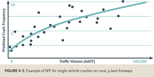
SPFs are a more reliable method to account for differences in traffic volume among sites because they reflect the nonlinear relationship between crash frequency and traffic volume. The SPF is an equation that represents a best-fit model that relates annual observed crashes to the site characteristics including annual traffic volume and other site characteristics. Typically, SPFs are estimated for a particular crash type for a type of facility (e.g., run-off-road crashes on rural two lane roads) using data from an entire jurisdiction or State. Figure 4-2 and Figure 4-3 show example SPFs where the points represent observed crashes at specific traffic volumes for individual sites, and the solid line represents the bestfit model (i.e., the SPF). If the relationship between exposure and crash frequency were linear, then the solid line would be a straight line instead of a curve. These two figures also demonstrate the nature of SPFs—each curve is different. For the rural, four lane freeways used in this example, multi-vehicle crashes rise exponentially with more traffic volume (Figure 4-2) but single-vehicle crashes behave differently; they level off with increasing levels of traffic volume (Figure 4-3).
An SPF produces the average number of crashes that would be predicted for sites with a particular set of characteristics. By comparing a site's observed number of crashes with the predicted number of crashes from an SPF, it may be possible to identify sites that experience more crashes than one would expect from a site with that particular set of characteristics. Sites where the observed number of crashes is larger than the predicted number of crashes from an SPF warrant further review and diagnosis. Two measures in Table 4-4, level of service of safety (LOSS) and the excess predicted average crash frequency using SPFs, use the observed crash frequency and predicted frequency from an SPF to identify sites with promise.
SPFs can be obtained in two ways:
1) SPFs can be developed from scratch using crash, roadway, and traffic volume data from roads and intersections in the State. This requires significant data to be collected on hundreds of sites. A statistical expert must use these data to develop SPFs that are tailor made for that State.
2) SPFs can be obtained from national resources, such as the HSM; then calibrated for the particular State of interest. This requires data to be collected on a smaller number of sites than is required for developing a new SPF.
The crashes predicted by the SPF are compared to the crashes observed on the State's roads, and an analyst calculates a calibration factor to adjust the SPF prediction appropriately for the State.
SPF development or calibration is typically handled by the State DOT. FHWA provides guidance on deciding between developing a new SPF or calibrating an existing one.10 States that decide to develop new SPFs can refer to guidance in a related FHWA publication.11 NCRHP provides guidance for those who decide to calibrate existing SPFs.12
The frequency of crashes per year that represents the combination of the predicted crashes and the observed crashes that actually occurred at the site.
The difference between the expected crashes and the observed crash frequency at the site.
Some States use Safety Analyst, a software tool from AASHTO, to identify sites that may benefit from a safety treatment.14 The following is an SPF from Safety Analyst that predicts the total number of crashes on rural multilane divided roads:
This is a relatively simple SPF where the predicted number of crashes per mile is a function of just AADT. For example, if the AADT is 45,000, then the predicted number of crashes for a one mile segment based on the SPF will be the following:
Bauer and Harwood17 provide a more complex SPF for fatal and injury crashes on rural two lane roads. This model provides a crash prediction that is more tailored to characteristics of the site, such as curve radius and vertical grade of the road:
![(Equation) NFI equals e to the power of the power of [negative 8.76 plus 1.00 times the natural log of AADT plus 0.044 times G plus 0.19 times the natural log of (2 times 5730 divided by R) times IHC plus 4.52 times (1 divided by R) times (1 divided by Lc) times IHC]. Where NFI equals fatal-and-injury crashes per mile per year, AADT equals annual average daily traffic (vehicles/day), G equals absolute value of percent grade; 0% for level tangents; ≥ 1% otherwise, R equals curve radius (ft); missing for tangents, IHC equals horizontal curve indicator: 1 for horizontal curves; 0 otherwise, LC equals horizontal curve length (mi); not applicable for tangents, ln equals natural logarithm function.](images/unit4_SPF_Example2.png)
Ideally, SPFs should be estimated using data from the same jurisdiction as the site(s) being studied.13 However, that may not always be possible due to the availability of data or lack of statistical expertise. In that case, the SPFs developed from another jurisdiction could be calibrated using data from the jurisdiction with the study sites.15
As previously discussed, RTM describes the situation when periods with relatively high crash frequencies are followed by periods with relatively low crash frequencies simply due to the random nature of crashes. Figure 4-4 illustrates RTM, comparing the difference between short-term average and long-term average crash history.16 Due to RTM, the short-term average is not a reliable estimate of the long-term crash propensity of a particular site. If an agency selects sites based on high short-term average crash history, crashes at those sites may be lower in the following years due to RTM, even if the agency does not install countermeasures at those sites.
If RTM is not properly accounted for, sites with a randomly high count of crashes in the short term could be incorrectly identified as having a high potential for improvement, and vice versa. In this case, scarce resources may be inefficiently used on such sites while sites with a truly high potential for cost effective safety improvement remain unidentified.
One approach to address RTM bias is to use the EB method. The EB method is a statistical method that combines the observed crash frequency (obtained from crash reports) with the predicted crash frequency (derived from the appropriate SPF) to calculate the expected crash frequency for a site of interest. This method pulls the crash count towards the mean, accounting for the RTM bias.
The EB method is illustrated in Figure 4-5, which illustrates how the observed crash frequency is combined with the predicted crash frequency based on the SPF.18 The EB method is applied to calculate an expected crash frequency or corrected value, which lies somewhere between the observed value and the predicted value from the SPF.
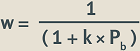
Mathematically, the expected number of crashes can be written as a function of the predicted value from the SPF and the observed crashes in the following ma5nner:
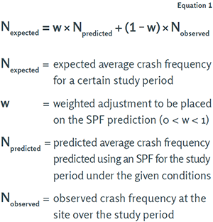
The weight w is a function of the predicted crash frequency (Npredicted) and a statistical parameter called the overdispersion parameter of the SPF. Procedures to estimate the expected average crash frequency are provided in Part B of the HSM. For example, if the observed crash frequency in a particular site was nine crashes per year, the predicted crash frequency from the SPF was 6.4 crashes per year, and the w was 0.3, then Nexpected will be as follows:
We can prioritize sites by calculating the difference between the EB expected crashes at a particular site and the predicted crashes from an SPF. By comparing EB expected crashes at a particular site instead of observed crashes, we account for possible bias due to RTM.
The first eight measures presented in Table 4-4 do not account for possible bias due to RTM. Measure 9 (probability of specific crash types exceeding threshold proportion) and measure 10 (excess proportion of specific crash types) are not affected by RTM unless they are based on short-term crash history. Measure 11 (expected average crash frequency with EB adjustments), measure 12 (EPDO average crash frequency with EB adjustment), and measure 13 (excess expected average crash frequency with EB adjustment) account for possible bias due to RTM using the EB adjustments.
The severity of crashes at a location can (and should) have a bearing on the priority of the site for safety treatment. Three of the measures in Table 4-4, measure 3 (EPDO average crash frequency), measure 4 (relative severity index), and measure 12 (EPDO average crash frequency with EB adjustment), directly account for crash severity. Measures 3 and 12 use the EPDO method, which converts all crashes to a common unit, namely property damage only (PDO) crashes. Using these measures, the analyst assigns points to each crash based on its crash severity level. A PDO crash typically receives one point and the points increase as the severity of the crash increases.
While other measures do not explicitly mention severity, analysts can adapt any of the measures to consider any severity level. For example, an analyst could use crash frequency and focus on the frequency of fatal and severe injury crashes to priority rank sites. It is important to note that the severity distribution of crashes may be a function of site characteristics including AADT. For example, sections with higher AADT values may be associated with lower speeds and consequently fewer severe crashes.
Diagnosis is the second step in the roadway safety management process, following network screening. Diagnosis is the process of further investigating the sites and issues identified from network screening. The intent of diagnosis is to identify crash patterns and the factors that contribute to crashes at the identified sites. Thorough diagnosis can also identify potential safety issues that have not yet manifested in crashes. Diagnosis often involves a review of the crash history, traffic operations, and general site conditions. While safety professionals could review these data from the office, a field visit provides the opportunity to observe road user behavior and site characteristics that are not available in the data. Sometimes, safety professionals may also conduct a field review at night or at other times that crash history has indicated to be of concern. It is important to diagnose the cause of the problem before developing potential countermeasures, just as a doctor examines symptoms to diagnose an underlying disease before formulating a prescription. Otherwise, resources may be misallocated if a countermeasure that does not target the underlying issues is selected and implemented.
The Haddon Matrix is a framework to identify possible contributing factors (e.g., driver, vehicle, and roadway/environment) which are cross-referenced against possible crash conditions before, during, and after a crash to identify possible reasons for events. This comprehensive understanding of crash contributing factors is important for the diagnosis of safety problems. An example of the Haddon Matrix is presented later under Countermeasure Selection on page 4-22.
The HSM recommends that diagnosis include the following parts:
An analyst can conduct a detailed review of the crash data from police reports to identify patterns. This could involve reviewing the crash type, severity, sequence of events, and contributing circumstances. Different visualization tools, such pie charts, bar charts, or tabular summaries, can be used to display various crash statistics. In addition to reviewing descriptive statistics, analysts can use various methods to identify underlying safety issues based on the recognition of crash patterns.
One method would be to identify locations that have a proportion of a specific collision type relative to the total collisions that is higher than some average or threshold proportion value for similar road types. Kononov found that looking at the percentage distribution of collisions by collision type can reveal the “existence of collision patterns susceptible to correction” that may or may not be accompanied by the overrepresentation in expected or expected excess collisions.19 Heydecker and Wu originally proposed this method.20 The method is identical for different location types. However, only similar location types should be analyzed together because collision patterns will naturally differ. For example, the collision patterns are different for stop-controlled intersections, signalized intersections, and two-lane roads, so the method would be applied separately to the three types of facilities and separately for urban and rural environments. Another method would be to investigate sites that experience a gradual or sudden increase in mean collision frequency.21
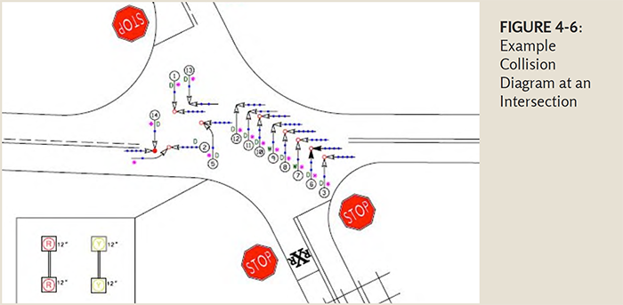
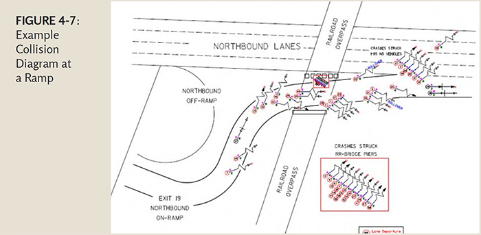
Following the detailed review of the crash data, the analyst can create collision diagrams, condition diagrams, and crash maps to summarize the crash information by location. A collision diagram is a tool to identify and display crash patterns. Many resources, including the HSM, provide guidance on developing collision diagrams. Examples of collision diagrams are shown in Figure 4-6 and Figure 4-7. Each crash at the site is displayed according to where it occurred, what type of crash it was, how severe it was, and various other characteristics. An analyst uses symbols to visually represent many of these characteristics.
Condition diagrams include a drawing with information about the site characteristics including information about the roadway (e.g., number of lanes, presence of medians, pedestrian and bicycle facilities, shoulder information), surrounding land uses, and pavement conditions. Condition diagrams can be overlaid on top of collisions diagrams to gain further insight to the crash patterns.
Crash mapping involves the use of geographic information systems (GIS) to integrate information from the roadway network with information from geocoded crash data. If the geocoded crash data are accurate, then crash mapping can provide valuable insights into crash locations and crash patterns.
This step involves a review of documented information about the site along with interviews of local transportation professionals to obtain additional perspectives on the safety data review from the previous step. Examples of supporting documentation include traffic volumes, construction plans and design criteria, photos and maintenance logs, weather patterns, and recent traffic studies in the area.
Field observations are useful for supplementing crash data and can help the analyst understand the behavior of drivers, pedestrians, and bicyclists. The first stage of the field investigation should be an on-site examination of a road user's experience. Those conducting the assessment should travel through the site at different times of the day using different modes of transportation (e.g., driving, walking, and bicycling). Assessors should observe the mix of vehicle traffic and other road users. They should also observe traffic movements, conflicts, and operating speeds. Those conducting the field review could determine whether the road and intersection characteristics are consistent with driver expectation and if roadside recovery zones are clear and traversable.
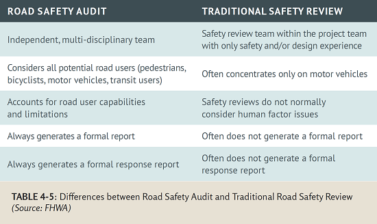
One method to assess field conditions is a road safety audit (RSA). This is the formal safety performance examination of an existing or future road or intersection by an independent, multidisciplinary team. An RSA qualitatively estimates and reports on existing and potential road safety issues and identifies opportunities for safety improvements for all road users. FHWA encourages States, local jurisdictions and tribal governments to integrate RSAs into the project development process for new roads and intersections and to conduct RSAs on existing ones.
The purpose of an RSA is to answer the following questions:
The multidisciplinary audit team consists of people who represent different areas of expertise, such as engineering (e.g., design, traffic, and maintenance), law enforcement, safety educators, public officials, community traffic safety advocates, and others. Any phase of project development (planning, preliminary engineering, design, construction) and any sized project from minor intersection and roadway retrofits to mega-projects are eligible for an RSA.
Most State DOTs have established safety review processes. However, RSAs and a traditional safety reviews are different. Table 4-5 shows the difference between an RSA and a traditional safety review.22
The International Road Assessment Programme (iRAP) conducts safety inspections on high-risk roads in more than 70 countries. The iRAP inspectors perform a detailed road survey, focusing on road attributes that are known to be associated with crash risk. These include intersection design, number of lanes, roadside hazards, and provisions for pedestrian crossings. The inspectors use these data to develop a star rating, which reflects the level of safety of the road, and provide detailed feedback to the government agency in the form of an assessment report. iRAP also provides a Road Safety Toolkit, which helps engineers, planners, and policy makers develop safety plans for all road users.23
After diagnosing the safety issues at the site, analysts select countermeasures to address the contributing factors for observed crashes. The first part of countermeasure selection is to identify countermeasures to target the underlying safety issues. Analysts can use tools like the Haddon Matrix and resources like the NCHRP Report 500 series to identify targeted countermeasures to address or mitigate underlying contributing factors.
The Haddon Matrix is a tool originally developed for injury prevention, but it is directly applicable to highway safety in both diagnosis and countermeasure selection.24 The Haddon Matrix is useful to gain a comprehensive understanding of crash contributing factors. Analysts can use the Haddon Matrix to identify human, vehicle, and roadway factors contributing to the frequency and severity of crashes prior to, during, and after the crash event. Then, analysts can identify targeted reactive and proactive countermeasures to address or mitigate the underlying contributing factors for the given site. Chapter 6 of the 1st edition of the HSM provides further discussion of the Haddon Matrix.
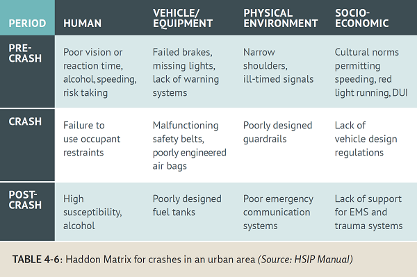
The Haddon Matrix is comprised of nine cells to identify human, vehicle, and roadway factors contributing to the target crash type or severity outcome before, during, and after the crash. Pre-crash factors speak to the factors or actions prior to the crash that contributed to the occurrence of the crash. Crash factors speak to those factors or actions that occurred at the moment of the crash. Post-crash factors speak to factors that come into play after the crash that affect the severity of the injuries or speed of response. Examples of human factors include fatigue, inattention, age, and failure to wear a seat belt. Vehicle factors include bald tires, airbag operations, and worn brakes. Examples of roadway factors include pavement friction, weather, grade, and limited sight distance.
Table 4-6 is an example application of the Haddon Matrix from the Highway Safety Improvement Program (HSIP) Manual for crashes in an urban area.25 The top-left cell identifies driver behaviors or characteristics that may contribute to the likelihood or the severity of a collision, such as poor vision or reaction time, alcohol consumption, speeding, and risk taking. These factors should be considered when selecting countermeasures. For example, based on these human factors, successful countermeasures may be those that improve visibility or reduce speeding. The matrix in its entirety provides a range of potential issues that can be addressed through a variety of countermeasures including education, enforcement, engineering, and emergency response solutions.
Diagnosing a roadway safety problem and identifying effective countermeasures is a skill developed through education, training, research, and experience. Many resources are available to help transportation professionals analyze and develop countermeasures. Since the transportation field continuously generates new knowledge and countermeasure approaches, it is important to stay informed of the available resources and tools.26
Some of the most useful resources and tools for countermeasure guidance and selection are listed below (alphabetically):
After identifying potential countermeasures to target the underlying issues, safety professionals must estimate the safety impact of countermeasures, individually and in combination. It is important to consider positive and negative safety impacts. Subsequent steps of the roadway safety management process (i.e., economic appraisal and project prioritization) include the consideration of other parameters, such as constructability, environmental impacts, and cost.
The agency that will be making the final decision on countermeasure selection should make sure to coordinate with other safety partners to ensure that the countermeasure is appropriate for all parties. For example, a DOT should coordinate with law enforcement and emergency response to make sure that a proposed engineering installation will interfere with enforcement activities or impede emergency responders.
FHWA provides an extensive selection of guidance on selecting and applying CMFs through the CMF Clearinghouse (www.cmfclearinghouse.org). They present answers to frequently asked questions, such as “How can I apply multiple CMFs?” and “How do I choose between CMFs in my search results that have the same star rating but different CMF values?” The website also houses an archive of annual webinars in which experienced CMF users talk about issues related to applying CMFs in real world situations.
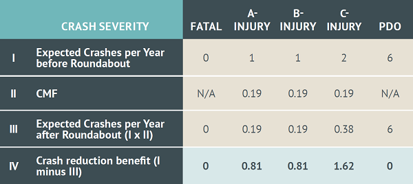
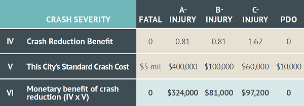
A city has a stop-controlled intersection with an expected crash frequency of 10 crashes per year, consisting of one A-injury crash, one B-injury crash, two C-injury crashes, and six PDO crashes.
The city is considering installing a roundabout at the intersection. Based on a search of the FHWA CMF Clearinghouse, they decide that they will use a CMF of 0.19 in the calculation of the crash reduction benefit.30 This CMF applies only to serious and minor injury crashes, so they do not use it to estimate any reduction to fatal or PDO crashes (see note).
They multiply the CMF by the expected crashes before roundabout installation to determine the expected crashes after installation:
Thus, the benefit of a roundabout installation is expected to be a reduction of 0.81 A-injury crashes, 0.81 B-injury crashes, and 1.62 C-injury crashes per year.
NOTE: A roundabout would also likely bring a reduction to fatal and PDO crashes (i.e., additional CMFs could be incorporated), but the example has been simplified to a single CMF for illustration purposes.
For infrastructure improvements, CMFs associated with different countermeasures provide a mechanism for determining the safety effect of different countermeasures. A CMF is a multiplicative factor used to compute the expected number of crashes after implementing a given countermeasure at a specific site.
For example, if the expected number of crashes without a countermeasure is 5.6 crashes per year, and the CMF for the particular countermeasure is 0.8, then the expected number of crashes with the countermeasure is:
5.6 crashes per year x 0.8 = 4.48 crashes per year
It is important to recognize that some countermeasures may decrease some types of crashes but increase other types. For example, installing a traffic signal would be expected to decrease severe collisions, such as right angle and left turn crashes, but it would be expected to increase less severe crashes, such as rear ends.
The CMF Clearinghouse and the first edition of the HSM provide CMFs for a variety of countermeasures.29 Only those CMFs that passed a set of inclusion criteria based on quality and reliability were included in the HSM. The CMFs in the clearinghouse are provided for any published study, regardless of quality, and are continuously updated based on the latest research. The CMFs in the clearinghouse are reviewed and given a star quality rating ranging from one to five stars, based on the quality of the study. Higher stars imply a better quality CMF.
CMFs should be applied to situations that closely match those from which the CMF was developed. Several variables can be used to match a CMF to a given scenario including roadway type, area type, segment or intersection geometry, intersection traffic control, and traffic volume. However, it is critical for practitioners to use engineering judgment when a CMF is not available for the situations encountered as there are some cases for which a CMF that was developed for different conditions might be the best available.
An economic appraisal of alternative countermeasures should be conducted to ensure that safety funds are being used as efficiently as possible. This appraisal helps transportation agencies achieve their desired safety performance the fastest and at the lowest possible cost. An agency can compare the benefits expected from the countermeasure to the estimated costs of the countermeasure.
Some safety countermeasures have a higher-cost value than others. Geometric improvements to the road, such as straightening a tight curve to reduce run-off-road crashes, tend to be very expensive. Installing a curve warning sign and in curve delineation may address the same problem, but at a much lower cost. Although both countermeasures address the same problem, the actual safety benefit may not be the same. Safety professionals take the relative costs and benefits into consideration when prioritizing among countermeasures. Part of calculating the cost of a countermeasure is considering how those costs vary over time, while taking into consideration any maintenance costs and long term effectiveness.
The primary benefit of a countermeasure is a reduction in crash frequency or severity. To estimate the safety benefits, a safety professional should use CMFs, such as those discussed in the countermeasure selection step. CMFs can be applied to the actual crashes or expected crashes based on the EB method. Expected crashes are preferred because they account for possible bias due to RTM. The estimated change in crashes represents the expected benefit from the countermeasure.
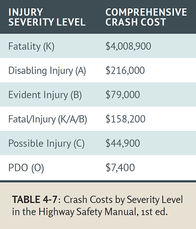
For each proposed countermeasure, the change in crash frequency and/or severity needs to be converted to monetary value, based on the monetary value of the type of crashes reduced. This monetary value is also called the crash cost. Crash costs are based on costs to society, such as lost productivity, medical costs, legal and court costs, emergency service costs, insurance administration costs, congestion costs, property damage, and workplace losses.31
The benefit from the countermeasure is the sum of the crash costs for crashes prevented by the countermeasure. Assigning costs to crashes is a topic that is under constant discussion and revision nationwide. States differ widely in the dollar amount that they assign to crashes, though all States apply higher values to more severe crashes. The CMF Clearinghouse provides a synthesis of crash costs that are used by various States.32
Additionally, the first edition of the HSM provided a list of crash costs by severity level (Table 4-7). However, since the publication of the first HSM in 2010, the USDOT has issued periodic recommendations that dramatically raised the values. For instance, the monetary value of a fatal crash was listed as $4 million in the HSM, but recommended as over $9 million in a 2013 policy memo from USDOT.33
Although countermeasures are primarily expected to reduce crashes, there might be other benefits, including reduced travel times or lower fuel consumption. For example, a roundabout can decrease total delay at an intersection if applied and configured properly. An AASHTO publication provides guidance on estimating these other non-safety benefits.34
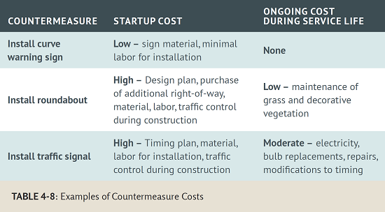
The costs of the proposed countermeasure include the startup cost and the ongoing operational and maintenance costs. These costs can usually be estimated based on costs of materials, labor cost per person-hour, cost of additional right-of-way, and past experience with similar countermeasures. Table 4-8 illustrates the types of startup and ongoing costs that would be incurred for various countermeasures.
Another important consideration when calculating the benefits and costs of a countermeasure is the length of time that the countermeasure will last. This is referred to as the service life. Countermeasures, such as road edgelines or pavement reflectors, will have a much shorter service life (e.g., three to five years) than countermeasures, such as traffic signal installation or sidewalk construction (e.g., 20 years or more). Many States have a standard list of the service life values used for common countermeasures. The CMF Clearinghouse provides a survey of service life values used by various States for many different countermeasures.35
The previous example showed that a city calculated a crash savings of 0.81 A-injury crashes, 0.81 B-injury crashes, and 1.62 C-injury crashes per year by installing a roundabout. The city has examined guidance from the HSM, guidance from USDOT, and experiences of other cities and States and determined a standard set of crash costs they will use for all benefit/cost calculations. They apply these costs to determine the monetary benefit of the expected crash reductions:
Thus, the city expects a total monetary benefit of $324,000 + $81,000 + $97,200 = $502,000 per year due to reduction in crashes.
The service life is used in the calculation of the present value of the benefits and costs of the proposed countermeasure. The calculation of present value includes a discount rate that reflects the time value of money (i.e., present dollars are worth more than future dollars). Present value of countermeasure benefits is calculated as follows:
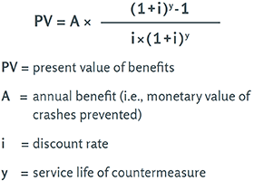
Calculating present value in this way assumes a uniform annual benefit. The HSIP Manual demonstrates how to calculate present value if the benefits or costs each year are not the same.36
The present value of annual costs (i.e., operational and maintenance costs) can be calculated in the same manner as for benefits. However, for costs, the final present value must also include the startup cost in the year of installation (see examples in Table 4-8).
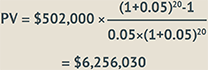
From the previous example, the city plans to install a roundabout and expects to see a benefit from crash reductions resulting in savings of $502,000 per year. They estimate that the roundabout will have a service life of 20 years and they determine that a discount rate of 5% is appropriate. They calculate the present value of benefits as:
There are several methods for using the values of estimated benefits and costs to evaluate the economic effectiveness of safety improvement projects at a particular site. In particular, these methods are useful in situations where a safety professional is considering several alternatives and desires to choose the countermeasure with the greatest benefit for the cost.
The HSIP Manual contains guidance on three methods—net present value, benefit/cost ratio, and cost effectiveness index.37 Net present value (NPV) is generally regarded as the most economically appropriate method, though the other two methods have certain advantages, as discussed below. The following sections provide quoted guidance from the HSIP Manual on economic appraisal.
The NPV method, also called the net present worth (NPW) method, expresses the difference between the present values of benefits and costs of a safety improvement project. The NPV method has two basic functions: 1) determining which countermeasure(s) is/are most cost efficient based on the highest NPV and 2) determining whether a countermeasure's benefits are greater than its costs (i.e., the project has a NPV greater than zero).
The formula for NPV is:

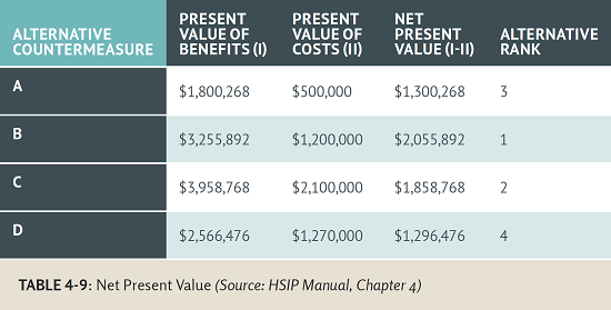
A countermeasure will result in a net benefit if the NPV is greater than zero. Table 4-9 summarizes the NPV calculations of four alternative countermeasures.
For Alternative A, the NPV can be calculated as follows:
The same calculation is performed for the other three countermeasure alternatives, and rank each countermeasure based on its NPV. As shown, all four alternatives are economically justified with a NPV greater than zero. However, Alternative B has the greatest NPV for this site based on this method.
The benefit/cost ratio (BCR) is the ratio of the present value of a project’s benefits to the present value of a project’s costs.
The formula for BCR is:

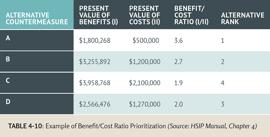
Table 4-10 shows an example of using BCR to prioritize four alternatives.
A project with a BCR greater than 1.0 indicates that the benefits outweigh the costs. However, the BCR is not applicable for comparing various countermeasures or multiple projects at various sites; this requires an incremental benefit/cost analysis.
An incremental benefit/cost analysis provides a basis of comparison of the benefits of a project for the dollars invested. It allows the analyst to compare the economic effectiveness of one project against another; however, it does not consider budget constraints. Optimization methods are best for prioritizing projects based on monetary constraints. An in-depth explanation of incremental benefit/cost analysis and an example is provided in Chapter 4 of the HSIP Manual.
When conducting a benefit/cost analysis, transportation professionals compare all of the benefits associated with a countermeasure (e.g., crash reduction), expressed in monetary terms, to the cost of implementing the countermeasure. A benefit/cost analysis provides a quantitative measure to help safety professionals prioritize countermeasures or projects and optimize the return on investment.
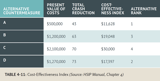
In situations where it is not possible or practical to monetize countermeasure benefits, transportation professionals can use the cost-effectiveness index method in lieu of the NPV or BCR. Cost-effectiveness is simply the amount of money invested divided by the crashes reduced. The result is a number that represents the cost of the avoided crashes of a certain countermeasure. The countermeasure with the lowest value is the most cost-effective and therefore ranked first.
Cost-Effectiveness Index = PVC/CR
PVC = Present value of project cost
CR = Total crash reduction
The Cost-Effectiveness Index is a simple and quick method that provides an indication of a project's value. Transportation professionals can use this formula and compare its results with other safety improvement projects. The Cost-Effectiveness Index method, however, does not account for value differences between reductions in fatal crashes compared to injury crashes, and whether a project is economically justified.38
Table 4-11 summarizes the calculations using the cost-effectiveness index method to rank alternative countermeasures, given the present value of the costs and the total crash reduction.
For Alternative A, calculate the cost-effectiveness index as follows:
Cost-effectiveness index = 500,000/43 = 11,628
Calculate the Cost-Effectiveness Index for the remaining alternatives and rank each countermeasure based on its Cost-Effectiveness Index value. With this method, the lowest index is the highest priority and therefore ranked first. Alternative A is ranked first, since it has the lowest cost associated with each crash reduction.
The above example uses the number of crashes to determine the cost-effectiveness index. Transportation professionals can use this same method using EPDO crash numbers, which has the advantage of considering severity.
If a transportation agency is considering installing countermeasures at one or more sites out of a group of potential sites, they will need to prioritize which projects they will implement. Ideally, the agency would implement all projects that bring a safety benefit (e.g., all those with a NPV greater than zero or a BCR greater than one). However, all agencies work within a limited budget and must prioritize where safety funds are spent.
The agency can use steps 1 through 4 of this process to determine which countermeasure(s) would be used at each potential treatment site and to conduct an economic appraisal of the expected effect of the countermeasure. The next step is to determine project priorities. The HSM discusses how projects can be prioritized by economic effectiveness, incremental benefit/cost analysis, or various optimization methods.
Projects can be prioritized by ranking projects or project alternatives by the economic appraisal values produced in step 4. An agency might select those projects with the highest NPV, the highest BCR, or the highest cost effectiveness index. When using NPV the goal of a safety professional should be to implement all projects that have an NPV greater than zero, since each one brings a safety benefit. However, this is not possible since funds are limited, thus the goal should be to implement the group of projects that have the greatest combined NPV when added together (NPV is an additive property). Maximizing the NPV of a group of projects is different from prioritizing projects with high NPV. In other words, it may be best to implement numerous low cost projects with low NPV than one high cost project with a high NPV—but not higher than the NPV of all the low cost projects added up.
This method involves ranking all projects with benefit cost ratio greater than 1.0 in increasing order of their estimated cost. An analyst calculates an incremental BCR as such:
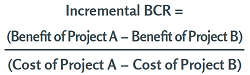
If the incremental BCR is greater than 1.0, the project with the higher cost is compared to the next project on this list; however, if the incremental BCR is less than 1.0, the project with the lower cost is compared to the next project on the list. This process is repeated and the project selected in the last pairing is the considered the best economic investment.
Optimization methods take into account certain constraints when prioritizing projects. Linear programming, integer programming, and dynamic programming (refer to Chapter 8, Appendix A, HSM, 2010) are optimization methods consistent with an incremental benefit/cost analysis, but they also account for budget constraints in the development of the project list. These optimization methods are more likely to be incorporated into a software package, rather than manually calculated. Multi-objective resource allocation is another optimization method. It incorporates nonmonetary elements (including decision factors not related to safety) into the prioritization process.
Safety professionals may use software applications to select and rank countermeasures. The SafetyAnalyst tool from AASHTO includes economic appraisal and priority ranking tools.39 The economic appraisal tool calculates the BCR and other metrics for a set of countermeasures. The priority-ranking tool ranks proposed improvement projects based on the benefit and cost estimates from the economic appraisal tool. The priority-ranking tool can also determine an optimal set of projects to maximize safety benefits.

A CMF can be obtained from a cross sectional model. Suppose the intent is to estimate the CMF for shoulder width based on the following SPF, which was estimated to predict the number of crashes per mile per year on rural two-lane roads in mountainous roads with paved shoulders (Appendix B of Srinivasan and Carter, 201144):
Where, AADT is the annual average daily traffic and SW is the width of the paved shoulder in feet. If the intent is to estimate the CMF of changing the shoulder width from three to six feet, then the CMF can be estimated as the ratio of the predicted number of crashes when the shoulder width is six feet to the predicted number of crashes when the shoulder width is three feet:
![CMF equals e to the power [0.8727 plus 0.4414 times the natural log of AADT divided by 10000 plus 0.4293 times (AADT divided by 10000) minus 0.0164 times 6] divided by the quantity of e to the power [0.8727 plus 0.4414 times the natural log of AADT divided by 10000 plus 0.4293 times (AADT divided by 10000) negative 0.0164 times 3].](images/unit4_CMFratio1.png)
This ratio simplifies to:
This CMF of 0.952 indicates that changing the shoulder width from three to six feet would be expected to reduce crashes (since the CMF is less than 1.0). Specifically, the expected change in crashes would be a 4.8% reduction (1.0 – 0.952 x 100 = 4.8).
However, it is important to recognize that this CMF of 0.952 is the midpoint in a range of possible values (i.e., the confidence interval). This range can be calculated by using the standard deviation of the CMF. In order to estimate the standard deviation, the standard error of the coefficient of SW is needed, which was reported to be 0.0015 in the original study. The high and low ends of the confidence interval are calculated using -0.0164+0.0015, and then using -0.0165-0.0015, and the difference between the two is divided by two. The equation is given below:
The approximate 95% confidence interval for the CMF is (0.952 - 1.96 x 0.004, 0.952 + 1.96 x 0.004), which translates to a range of 0.944 to 0.960. Since the entire 95% confidence interval is below 1.0, the CMF is statistically significant, thereby indicating that widening the shoulder from three to six feet is very likely to reduce crashes.
This example is an illustration of an EB before-after evaluation that was conducted as part of NCHRP Project 17-35.51 The countermeasure was a change from permissive to protected-permissive left turn phasing at signalized intersections in North Carolina. Data from twelve locations were used in this evaluation. A reference group of 49 signalized intersections was identified for the development of SPFs. The analysis looked at total intersection crashes, injury and fatal crashes, rear end crashes, and left turn opposing through (LTOT) crashes. In this example, only the data for LTOT crashes will be used.
The SPF for LTOT crashes based on the data from the reference group was:
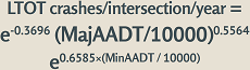
Where, MajAADT is the major road AADT and the MinAADT is the minor road AADT. The overdispersion parameter (k) for this SPF was 0.5641.
In the first site of this study, there were 10 observed crashes in the before period (Xb), and the predicted number of crashes from the SPF in the before period was 5.535 (Pb). The formula for obtaining the EB estimate of the expected crashes in the before period (EBb) is as follows:
Where, Xb is the observed crashes in the before period, and w is the EB weight that is calculated as follows:
Where, k is the overdispersion parameter for the estimated SPF.
In this example:
The EB estimate of the crashes in the before period (EBb) = 5.535*0.243 + 10*(1-0.243) = 8.917 crashes.
The predicted number of crashes from the SPF in the after period was 11.391 (Pa).
The formula for the EB expected number of crashes that would have occurred in the after period had there been no countermeasure is given by:
In this example, the EB expected number of crashes in the after period had the countermeasure not been implemented (π) is equal to:
The variance of this expected number of crashes is also estimated in this step:
Where, Pa is the SPF predictions in the after period. In this example, the variance of ππ is estimated as follows:
This process was repeated for all 12 sites. Based on the data for all the 12 sites that were used in the evaluation, the actual crashes in the after period were 115, the EB expected crashes had the countermeasure not been implemented was 131.933 with a variance of 140.080.
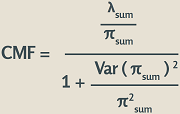
The formula for the CMF and its standard deviation (StDev) are as follows:
![standard deviation of the CMF equals the square root of [CMF squared times (variance of lambda sum divided by lambda sum squared) times (variance of pi sum divided by pi sum squared)] divided by [1 plus (variance of pi sum divided by pi sum squared)] squared.](images/unit4_CMF_StDev_squareroot1.png)
Where, λsum is the total number of crashes that occurred in the after period, for all the treated sites in the sample, πsum is the total number of expected crashes in the after period had the countermeasure not been implemented, and Var represents the variance. Since crashes are assumed to be Poisson distributed, Var(λsum) is usually assumed to be equal to λsum. So, (Var(λsum))/(λsum2) will be equal to 1/λsum.
In this example, the overall CMF was calculated as:
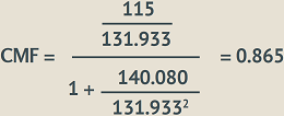
This CMF of 0.865 indicates that the countermeasure (changing from permissive to protected-permissive left turn phasing) would decrease crashes, since the CMF is less than 1.0. It would be expected to decrease crashes by 13.5% (1.0 - 0.865 x 100 = 13.5).
Again, it is important to recognize that the CMF is the midpoint of a range of possible values (i.e., the confidence interval). The standard deviation of the CMF can be estimated as follows:
![standard deviation of the CMF equals the square root of [0.865 squared times (1 divided by 115) times (140.080 divided by 131.933 squared)] divided by [1 plus (140.080 divided by 131.933 squared)] squared which equals 0.111.](images/unit4_CMF_StDev_squareroot2.png)
Based on this standard deviation of the CMF, the approximate 95% confidence interval is (0.865-1.96×0.111, 0.865+1.96×0.111), which translates to a range of 0.647 to 1.083. Since this confidence interval includes values greater than 1.0, the CMF is not statistically different from 1.0 at the 95% confidence level. This indicates that there is less confidence that this countermeasure will reduce crashes compared to a countermeasure whose CMF is significantly different from 1.0.
Once a countermeasure has been implemented at a site, or group of sites, it is important to determine whether it was effective in addressing the safety problem. For a safety professional to evaluate the countermeasure, he or she must determine how the countermeasure affected the frequency, type, and severity of crashes. For example, did the installation of a roundabout reduce the frequency of angle crashes? If so, by how much? Did it cause an increase to any other types of crashes? A countermeasure evaluation can result in a CMF for the countermeasure, which quantifies the effect on crashes (see CMF discussion in Step 4).
Two documents entitled A Guide to Developing Quality Crash Modification Factors40 (from FHWA) and Recommended Protocols for Developing Crash Modification Factors41 (from NCHRP) provide guidance on the different methods for conducting evaluations. The following is an overview of study designs and methods for conducting evaluations.
Study designs fall into two broad categories—experimental and observational. Experimental studies are conducted when sites are selected at random for treatment. There is general consensus that experimental studies are the most rigorous way to establish causality.42 In contrast, observational studies are conducted when sites are not selected as part of an experiment but selected for other reasons including safety. Truly experimental studies are not common in road safety partly because of potential liability considerations (i.e., a random selection may result in an agency being held liable for failing to treat some sites that have demonstrated high crash history). Observational studies are more common in countermeasure evaluations because most transportation agencies prioritize installation sites based on some kind of past safety performance (see Step 1, Network Screening).
Observational studies of countermeasures can be broadly classified into cross-sectional studies and before-after studies. In cross-sectional studies, an analyst compares a group of sites with a certain feature to a group of sites without that feature. For example, an analyst might compare the safety performance of a group of stop-controlled intersections to that of a group of yield-controlled intersections to determine the effect of the type of traffic control on crashes. Cross-sectional studies can also be thought of as “with/without” studies. In before-after studies, an analyst takes a group of sites and compares the safety performance in the period before a countermeasure is implemented to the period after the countermeasure is implemented. For example, in a before-after study, an analyst could evaluate the effect of converting a stop-controlled intersection to a roundabout by comparing safety data before the roundabout conversion to the safety data afterwards.
CMFs that result from cross-sectional studies are not considered to be as robust as those resulting from a before-after study. In a typical before-after study, an analyst deals with same roadway unit located in a particular place, most likely used by the same road users during the before and after period. Since most of these factors can be assumed to be constant or almost constant in the before and after periods, they are less likely to cause significant biases. On the other hand, “cross-sectional studies compare different roads, used by different road users, located at different places and subject to different weather conditions. Besides, these roads will differ in very many other ways that are not measured.”43 However, there are issues in both types of studies that need to be addressed, and they are briefly discussed below.
Analysts use cross-sectional studies to compare the safety of a group of sites with a feature with the safety of a group of sites without that feature. The resulting CMF can be derived by taking the ratio of the average crash frequency of sites with the feature to the average crash frequency of sites without the feature. For this method to work, the two groups of sites should be similar in their characteristics except for the feature. In practice, this is difficult to accomplish and multiple variable regression models are used. These cross-sectional models are also called SPFs. The coefficients of the variables from these equations are used to estimate the CMF associated with a treatment.
Guidance from FHWA on developing CMFs says that “the basic issue with the cross-sectional design is that the comparison is between two distinct groups of sites. As such, the observed difference in crash experience can be due to known or unknown factors, other than the feature of interest. Known factors, such as traffic volume or geometric characteristics, can be controlled for in principle by estimating a multiple variable regression model and inferring the CMF for a feature from its coefficient. However, the issue is not completely resolved since it is difficult to properly account for unknown, or known but unmeasured, factors. For these reasons, caution needs to be exercised in making inferences about CMFs derived from cross-sectional designs. Where there are sufficient applications of a specific countermeasure, the before-after design is clearly preferred.”45

One way to account for some of the limitations of cross-sectional regression models is to use the propensity scores-potential outcome method. This method uses the “individual traits of a site to calculate its propensity score, defined as a measure of the likelihood of that site receiving a specific treatment. Sites with and without the treatment are then matched based on their propensity scores.”46 The matched data are then used to estimate a cross sectional regression model. The propensity score method has been shown to reduce selection bias by accounting for the non-random assignment of treatment sites.47 Recently, the propensity score method is starting to be used in place of traditional cross-sectional methods to conduct evaluations.48
Other types of cross-sectional methods include case control and cohort methods. “Case-control studies select sites based on outcome status (e.g., crash or no crash) and then determine the prior treatment (or risk factor) status within each outcome group.”49 Another critical component of many case-control studies is the matching of cases with controls in order to control for the effect of confounding factors. In cohort studies, sites are assigned to a particular cohort based on current treatment status and followed over time to observe exposure and event frequency. One cohort may include the treatment and the other may be a control group without the treatment. The time to a crash in these groups is used to determine a relative risk, which is the percentage change in the probability of a crash given the treatment.50
An analyst can use a before-after study to evaluate a countermeasure by comparing the crashes before the countermeasure was installed to the crashes after installation. This study design is advantageous because the only change that has occurred at the site is the countermeasure installation (assuming the analyst has researched the site histories to discard any sites at which other significant changes occurred).
There are issues for consideration with this study design as well. The analyst must know when the countermeasure was installed and must have data, such as crash and traffic volume, available in the before and after periods. For high-cost, high-profile countermeasures, such as road widening or traffic signal installation, the installation records will be readily available. However, for low-cost countermeasures, such as sign installations, there may be little to no documentation on when they were installed.
The analyst might simply compare the number of crashes per year before the countermeasure to the number of crashes per year after the countermeasure, known as a simple or naïve before-after evaluation. Although a simple before-after evaluation can be done easily using only crash data, it is prone to significant bias. One of the most influential biases for this method is the possible bias due to RTM. As discussed earlier, RTM describes a situation in which crash rates are artificially high during the before period and would have been reduced even without an improvement to the site. Programs focused on high-hazard locations are vulnerable to the RTM bias. This potential bias is greatest when sites are chosen because of their extreme value (e.g., high number of crashes or crash rate) in a given time period. A simple before-after evaluation has a high likelihood of showing a much greater benefit from the safety treatment than actually occurred.
As discussed earlier under the network screening section, the EB method is one of the methods that has been found to be effective in dealing with the possible bias due to RTM. The following steps are needed to conduct an EB before-after evaluation:
The expected number of crashes without the treatment along with the variance of this parameter and the number of reported crashes after the treatment is used to calculate the CMF and the standard deviation of the CMF. This procedure is repeated for each treated site. Once CMFs have been calculated for each individual site in a group of treated sites, the CMFs can be combined to calculate the overall effectiveness of the countermeasure. More details on this procedure are provided in the previously mentioned guidance documents.52,53
In some cases, treatments may be installed system-wide for a particular type of facility. For example, a jurisdiction may decide to increase the retroreflectivity of all their stop signs. Since sites are not specifically selected based on their crash history, the bias due to RTM is minimal. However, it is still necessary to account for changes in traffic volume and other trends. To evaluate the safety of such installations, an EB method could still be used, and while a reference group is not necessary, a comparison group is necessary in order to account for trends. SPFs can be estimated using the before-data from the treatment sites and these SPFs can be used to account for changes in traffic volumes. In addition, SPFs could be estimated for a group of comparison sites and the annual factors from these SPFs can be used to account for trends. Further details about such evaluations can be found elsewhere.54
System-wide is a general term that refers to treating safety issues across an entire transportation system using policies or campaigns. Systemic is a more specific term that refers to identifying a subset of a transportation system based on risk factors and implementing safety efforts that address the particular characteristics of that subset. See more information on the systemic approach.
System-level safety management involves addressing road safety issues that affect the broad transportation system, as opposed to treating specific high priority sites. The size and scope of the transportation system depends on the agency or jurisdiction. For a State DOT, the transportation system would consist of all State-owned roads, signals, bridges, and other features across the entire State, whereas the transportation system for a town would consist of a much smaller area and roadway network. Road safety at a system-level often has to do with policies, whether design policies for the construction and operation of roads and intersections, driver policies for licensing, or vehicle policies that require certain safety technologies. Other system-level efforts would include broad media or enforcement campaigns.
Recall that Chapter 10 presented road safety management in terms of three general components:
This chapter will discuss how each of these components can be addressed at a system-level.
To identify safety problems on a system-level, safety professionals analyze safety data that apply to the entire jurisdiction. They examine crash data and link crashes to other safety data to determine the nature and locations of safety problems. Problem identification on a system-level involves identifying crash trends and using risk-based methods to prioritize safety efforts.
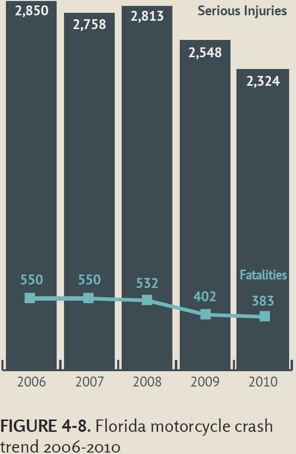
The State of Florida examined its crash data to identify emphasis areas in the development of their SHSP in 2012. One area that continued to be a focus was motorcyclist safety. The data indicated that crashes involving motorcycles had decreased somewhat during the time period analyzed (2006 to 1010) but remained a significant portion of the crashes on Florida roads. Florida's safety professionals recognized that since Florida hosts numerous national motorcycle events, the state's SHSP should have motorcycle safety as an emphasis area.
A statewide-coordinated safety plan that provides a comprehensive framework for reducing highway fatalities and serious injuries on all public roads.
Safety professionals can examine crash types and contributing factors to determine the nature of crashes within their agency's jurisdiction. This type of examination may reveal crash trends, such as those related to alcohol involvement, seat belt use, driver age, or vulnerable road users. For example, crash data might show that crashes involving unbelted occupants have been increasing over the past several years, or it might show that the number of crashes involving unbelted occupants is significantly higher than other nearby agencies, such as adjacent counties or States. This would lead an agency to consider how to increase seat belt use, perhaps through media campaigns, increased enforcement, or educational campaigns in schools. This type of agency-wide analysis of crash data can demonstrate broad scale trends that need to be addressed through broad scale efforts.
It is important that safety professionals are specific when identifying safety problems in crash trends. For example, “crashes involving teen drivers” is not defined well enough, because the causes of crashes for 16 year-olds is markedly different from those of older, more experienced teens. Crashes in which teens are victims of other drivers' errors require different solutions from those where the teen was at fault. Similarly, the cause of crashes depends greatly on the specific time, place and driving environment. A better target crash type would be “crashes occurring between 7-9 a.m. involving 16-year old drivers.”
A good example of identifying safety problems from crash type trends can be seen in how States develop strategic highway safety plans (SHSPs). The development of a SHSP involves the identification of safety problems on the State and local roads. A State analyzes safety data to determine the priorities, referred to as emphasis areas. The analysis can involve an examination of crash proportions between categories of crashes, crash trends, crash severity (e.g., fatal and serious injury), or more advanced crash modeling techniques. As presented in the call-out boxes, Ohio and Florida conducted analyses of their crash data and identified areas of concern.

Ohio developed a SHSP in 2014 in which they identified fifteen emphasis areas. One of the emphasis areas was the safety of older drivers (65 and older). The crash data showed that older driver-related crashes accounted for 18% of highway deaths and 16% of serious injuries. They recognized that these numbers would likely increase with an aging population. The crash trends over the time period examined (2003 to 2013) showed a slight upward trend to older driver serious injuries and a slight downward trend to older driver fatalities. This contrasted to other types of crashes that experienced significant declines. These reasons motivated Ohio to make older driver safety an emphasis area in their 2014 SHSP.
Chapter 11 presented various methods of selecting high priority sites through a process of network screening based on crash data. Many safety professionals recognize that this process of identifying specific locations using past crash data does not adequately address the fact that there may be locations that pose a safety threat but have not yet experienced many (or any) crashes. This recognition led to an increased use of risk-based prioritization, also called the systemic approach.55
In this approach, a transportation agency identifies priority locations based on the presence of risk factors rather than crashes. In the medical field, doctors pay attention to factors that may elevate a person's risk for disease. A history of smoking, poor eating habits, and a lack of exercise may indicate a higher-than-average risk for heart disease, even if the person has not yet experienced heart problems. Similarly, a section of road with certain characteristics, such as sharp curvature, old pavement, or lack of visibility, may be at risk for run-off-road crashes, even if none have occurred yet. Agencies can be proactive in their approach to safety management by identifying and treating these sites before crashes occur. These treatments are often low cost, such as signs and markings, so many systemic-identified locations can be treated within an agency's limited budget.
The process of identifying road or intersection characteristics that increase the risk of crashes and selecting locations for safety treatment based on the presence of these risk factors.
An agency using the systemic approach selects the focus crash type(s) and identifies risk factors associated with the focus crashes. Risk factors are site characteristics (e.g., design and operational features) that are common across locations with the focus crash type(s). The agency can identify risk factors by analyzing crash data from their jurisdiction or by reviewing previous research studies. Using the list of risk factors as a guide, the agency identifies a list of sites with those specific characteristics, and then develops targeted treatments to address or mitigate the specific risk factors. The agency can apply crash history and other thresholds to reduce the list of sites based on available resources and program objectives.
The systemic approach has two attractive features. First, an agency can employ the systemic approach even for roads or intersections where crash data are not fully available (e.g., where location accuracy is questionable or underreporting is a problem). For instance, locating crashes accurately and precisely in rural areas or on non-State owned urban roads can be difficult. Second, the systemic approach is useful for treating safety issues where crashes are highly dispersed, such as on rural or low volume roads. Specifically, agencies can use the systemic approach to address existing and potential safety issues across a large portion of the network (e.g., shoulder rumble strips on all rural, two-lane roads with a certain shoulder width and traffic volume level).
After safety professionals analyze data and identify safety problems, they must develop potential strategies to address the problems. It is important to engage safety stakeholders and other partners when selecting potential strategies as they may provide unique perspectives. Safety professionals should seek to involve local officials, citizens, and safety partners to produce effective multidisciplinary strategies. For example, addressing a particular safety problem with law enforcement and education can be far more economical than implementing a multimillion-dollar engineering fix. On the other hand, law enforcement tends to be effective only during the time in which it is active, so a more permanent engineering measure may be needed in some cases. It is often the case that a combination of strategies is necessary to effectively address the multitude of contributing factors.
On a system level, agencies must think broadly across the many disciplines represented by those who have a stake in road safety. Potential strategies might address infrastructure policies and practices (e.g., design standards, speed limits, etc.) or they may be directed at specific population focused efforts (e.g., seat belt laws, helmet laws, young driver restrictions, etc.).
Just as the identification of problems was based on safety data, so too must the development and selection of strategies be driven by the data. If an agency identified concerning trends in certain types of crashes, then they should further examine the crash data to determine how best to address the safety problem. For example, Figure 4-9 shows an example of alcohol-related crashes where an agency identified a spike in frequency (or high pole) of crashes occurring near 2:00 AM. Further examination revealed that bars in that jurisdiction closed at 2:00 AM. This could lead to potential strategies, such as increased enforcement of impaired driving at that time of night and in the vicinity of bars.
The Thurston County Public Works Department in Washington conducted a systemic safety analysis for their road network. Based on a review of severe crashes, Thurston County decided to focus on roadway departure crashes in horizontal curves on arterial and collector roadways when it found that:
Thurston County accessed an inventory of their roads and intersections through a database maintained by the Statewide County Road Advisory Board. In addition, Thurston County assembled crash data for the 2006-to-2010 timeframe from the Washington State DOT crash database. They linked the road, intersection, and curve data with crash data and used these data to identify risk factors. Thurston County assembled a list of 19 potential risk factors and then performed a descriptive statistics analysis to identify 9 risk factors for use in screening and prioritizing candidate locations. The identified risk factors were:
Thurston County decided that a risk factor could be worth one point or a one-half point. Those factors present in at least 30% of the severe (fatal and injury) crashes and overrepresented by at least 10% (when comparing the proportion of all locations with the proportion of severe crash locations) were used as a guideline to have a high confidence and assigned one point in the risk assessment process. The risk factors that had a lower confidence in their relative data were assigned one-half point.
Thurston County then tallied the number of risk factors present for each of the curves. The risk factor totals for the ten curves with the highest scores ranged from 4.5 to 6.0. All 270 signed curves were prioritized for potential low cost safety investments. They identified the following low-cost, low-maintenance countermeasures with documented crash reductions to implement at the selected locations:
Systemic analysis provided Thurston County a proactive, data-driven, and defensible approach to identifying curves for improvement prior to a severe crash occurring, rather than reacting after an incident has occurred.56
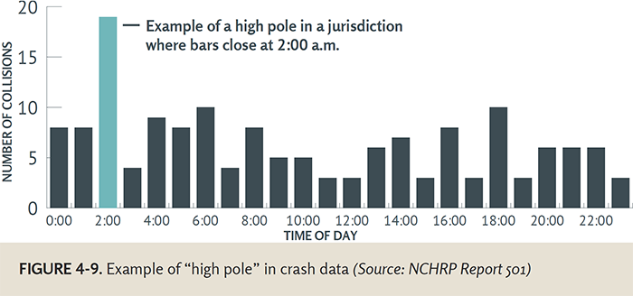
It is also important to use the data to determine the necessary scope of the intervention. If the data show that the problem exists year-round, then the solution needs to match that. For example, a “safe ride program” for drinkers to get home on New Year's Eve is not going to significantly impact the problem of impaired driving overall.
Safety professionals must identify and target road user behaviors that contribute to the identified safety problem. The target behavior should be specific. For example, “safe driving” is not a specific behavior that can be changed because it involves a number of different behaviors. However, “speeding on Main Street” is a specific behavior that can be targeted. It is also important to consider the factors influencing this behavior. Why are people speeding on Main Street? Which social, cultural, or environmental factors are influencing this behavior? Does it vary by time of day or week, perhaps reflecting the kind of drivers who are speeding?
After identifying motorcyclist safety as an emphasis area in their 2012 SHSP, Florida identified a list of strategies to address motorcyclist safety. Example strategies include:
Critical thinking is needed to develop effective solutions to the safety problems at hand. Analysts should look for characteristics of crash trends that could be addressed by practical strategies. An NCHRP report on an integrated safety management process states that safety professionals should use safety data to perform “further analyses of those characteristics that are found to be significantly or practically over-represented on a percentage or rate basis.”57 The report gives a set of guidelines to be considered in analyzing crash data to identify trends and develop potential safety strategies:
Many system-level safety strategies focus on behaviors of drivers and other road users. Resources like Countermeasures That Work provide a useful listing of potential safety strategies for system-level safety management.59 The excerpt from Countermeasures That Work in Figure 4-10 gives a list of potential strategies for addressing speeding-related crashes, from either laws, enforcement, penalties and adjudication, or communications and outreach. The list also includes an indication of the effectiveness, cost, current usage, and time of each strategy, which are all important considerations when selecting safety strategies to implement.
If the agency identifies safety problems from a systemic analysis, the potential safety strategies should address the types of crashes that were related to the roadway characteristic risk factors. These strategies may often be engineering improvements related to the risk factors. For example, if an examination of crash trends may highlight run-off-road crashes, and a systemic analysis would identify the type(s) of road on which run-off-road crashes are likely to occur. Table 4-12 shows a list of potential safety strategies that could be implemented for engineering treatments for a run-off-road crash problem. In a systemic approach, these engineering treatments would be implemented across some or all roads meeting the risk factors that increase the likelihood of run-off-road crashes.
SHSPs provide many good examples of system-level strategies that address safety problems identified through analysis of crash and other safety data. The previous section showed how Ohio and Florida had identified safety priorities on older drivers and motorcyclists, respectively. The SHSPs from these States also demonstrated the types of safety strategies each State intended to pursue to combat the safety problems in these areas.
A transportation agency must determine which of the potential strategies they will implement to address the identified safety problems. Since system-level safety solutions can involve broad changes to policies, design practices, or jurisdiction-wide road user behavior, there are different issues to consider compared to implementing a safety countermeasure at a specific location. Many more people will be affected by the system-level changes. This carries great promise in that safety might be improved across an entire system, but it also carries unique challenges.
Agencies will need to consider the following questions when selecting strategies to implement:
Communication is critically important for system-level safety strategies. Both the general public and road users affected by the strategy must understand the benefits. Other public agencies may need to integrate their efforts with the proposed safety strategy. Administrators, lawmakers, and other key decision-making personnel must understand how the strategy will improve road safety for their constituency and bring an overall financial benefit. Unit 5 provides more discussion on communication, marketing, and outreach for agencies who seek to implement system-level safety strategies.
Evaluating a system-level strategy (e.g., program or intervention) to determine its effectiveness is a critical but often overlooked step. The transportation agency in charge should evaluate the effect of the safety strategy using good quality data; ideally the same type of data that was used to identify the safety problem initially. If a program or intervention is not effective, the overseeing agency should consider why this might be the case. Can the program be improved, or should other approaches be considered instead? If successful, how can the intervention be institutionalized to ensure long term support (and therefore lasting change)? Finally, it is important to remember that success or failure in one location does not guarantee the same results at a different location.
Ohio identified three strategies to address the older driver emphasis area in their 2014 SHSP:
The following provides an example of using system-level safety management to address a specific problem. This example demonstrates the three general components of safety management presented in this unit.
County A noticed a large number of crashes involving 16-17 year old drivers occurring weekdays between 11:00am and 1:00pm. Neighboring counties have not experienced this problem. County officials coordinate with school district staff to tackle this issue.
In exploring the problem, the officials discover that County A is the only jurisdiction that has an open campus lunch policy allowing students to leave school during their lunch period. Allowing teens to leave campus during lunch means there are many young, inexperienced drivers on the roads at the same time. They may be carrying additional passengers which research has established leads to an increased risk of a fatal crash.60,61 The brief lunch period also results in pressure to get back in time for the next class. Combined, these factors lead to a risky driving situation and an increased risk of crashing.
In this situation, an informational approach that simply tells teenagers about the problem would likely not make a difference. Teens are not crashing because they lack information about the importance of safe driving or the consequences of unsafe driving. Teens are crashing largely because they lack the driving experience that equips most drivers to intuitively/near instantaneously do the things necessary to avoid crashing. Because of this, changing the environment is more likely to be effective.
The officials recognize that eliminating the policy that allows students to leave campus during lunch would lead to a reduction in crashes during this time. This policy would eliminate exposure to the risky driving situation and reduce the potential for crashes.
The school districts accordingly eliminate the policy allowing students to leave campus during lunch. They recognize that this policy change should be evaluated to determine its safety effect. Crash data would be needed to examine whether the closed school lunch policy has an effect on weekday crashes between 11:00am and 1:00pm. However, it will take many years to accumulate enough data for this evaluation. In this example, there is a proxy measure that can be used in the interim. A before and after observational survey with an appropriate control could quantify the number of students leaving campus during lunch before and after the change. In this case the officials know that the proxy measure (reduced driving from 11:00am to 1:00pm) is a guaranteed indicator of crash reduction for this specific problem. However, it is not often the case that proxy measures are so closely aligned to the outcome of interest.

Solving road safety problems requires a comprehensive process to identify safety problems, develop potential safety strategies, and select and implement those strategies. To get the most effective results, this process must be based on solid safety data, particularly good quality crash data. The methods of undertaking the safety management process will depend on the scope of the effort.
Safety management of individual sites involves a six-step process of screening the network for high-priority sites, diagnosing the safety issues at those sites, selecting appropriate countermeasures, conducting an economic appraisal for all options, prioritizing the countermeasure projects based on estimated costs and benefits, and evaluating the countermeasure performance afterwards. Safety management at a system-level involves identifying safety problems by examining crash trends or using a systemic approach to identifying high-risk road characteristics. State agencies who are developing system-wide safety strategies must examine the data trends and the road users involved. They must consider factors, such as how system-wide policies and programs will be accepted by the public and who will be the partners to involve in implementing the safety strategy.
RSPCB Program Point of Contact
Felix Delgado, FHWA Office of Safety
Felix.Delgado@dot.gov
FHWA Office of Safety
Staff and Primary Work Responsibilities
FHWA Office of Safety
Safety and Design Team
FHWA Resource Center